

How To Draw An Roc Curve
Written by MMA
on
12 mins to read.
How to plot ROC bend and compute AUC by hand
Assume nosotros have a probabilistic, binary classifier such equally logistic regression.
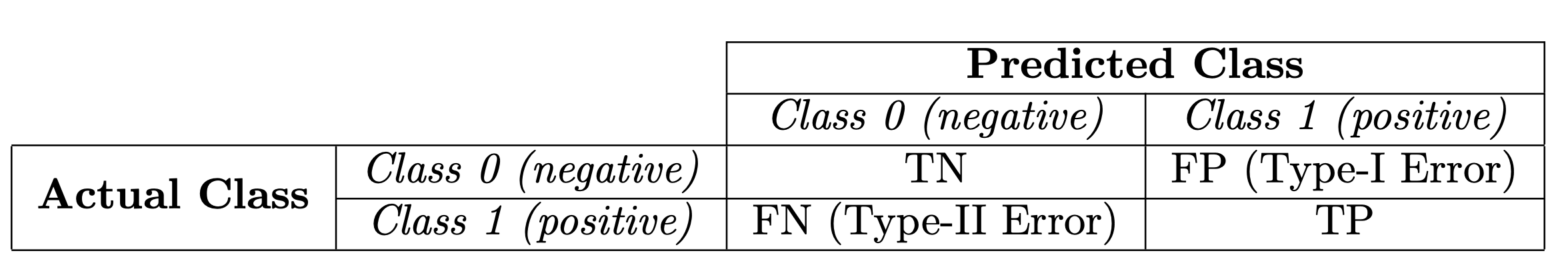
Before presenting the ROC curve (Receiver Operating Characteristic curve), the concept of confusion matrix must be understood. When we brand a binary prediction, there tin be 4 types of outcomes:
- We predict 0 while the true grade is really 0: this is chosen a Truthful Negative, i.e. we correctly predict that the class is negative (0). For example, an antivirus did not find a harmless file every bit a virus .
- We predict 0 while the true course is actually i: this is called a Imitation Negative, i.e. we incorrectly predict that the course is negative (0). For example, an antivirus failed to notice a virus.
- Nosotros predict ane while the true class is actually 0: this is called a False Positive, i.e. we incorrectly predict that the form is positive (1). For example, an antivirus considered a harmless file to exist a virus.
- We predict 1 while the true grade is actually i: this is chosen a True Positive, i.e. we correctly predict that the class is positive (1). For example, an antivirus rightfully detected a virus.
To go the defoliation matrix, nosotros get over all the predictions made past the model, and count how many times each of those 4 types of outcomes occur:
Since to compare two different models it is ofttimes more than convenient to have a single metric rather than several ones, we compute two metrics from the confusion matrix, which we will later combine into one:
-
True positive charge per unit (TPR), a.k.a. sensitivity, hit rate, and recall, which is defined equally $\frac{TP}{TP+FN}$. This metric corresponds to the proportion of positive data points that are correctly considered equally positive, with respect to all positive data points. In other words, the higher TPR, the fewer positive data points we will miss.
-
False positive rate (FPR), a.k.a. simulated alarm charge per unit, fall-out or one - specificity, which is defined as $\frac{FP}{FP+TN}$. Intuitively this metric corresponds to the proportion of negative data points that are mistakenly considered as positive, with respect to all negative data points. In other words, the higher FPR, the more negative data points will be missclassified.
To combine the FPR and the TPR into ane single metric, nosotros starting time compute the two onetime metrics with many unlike threshold (for example $0.00, 0.01, 0.02, \cdots , one.00$) for the logistic regression, then plot them on a single graph, with the FPR values on the abscissa and the TPR values on the ordinate. The resulting curve is called ROC curve, and the metric nosotros consider is the AUC of this curve, which nosotros telephone call AUROC. Threshold values from 0 to 1 are decided based on the number of samples in the dataset.
AUC is probably the second most popular 1, after accuracy. Accurateness deals with ones and zeros, meaning you either got the class label right or you didn't. But many classifiers are able to quantify their uncertainty virtually the answer by outputting a probability value. To compute accurateness from probabilities you need a threshold to decide when zero turns into i. The about natural threshold is of form 0.5. Let'due south suppose you have a quirky classifier. Information technology is able to become all the answers right, but it outputs 0.7 for negative examples and 0.9 for positive examples. Clearly, a threshold of 0.five won't get yous far here. Simply 0.8 would be but perfect.
That'due south the whole bespeak of using AUC - it considers all possible thresholds. Various thresholds result in dissimilar truthful positive/false positive rates. Every bit you subtract the threshold, y'all get more than truthful positives, but besides more false positives.
The following figure shows the AUROC graphically:
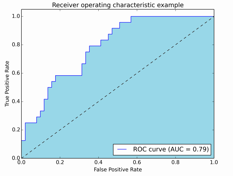
AUC-ROC bend is basically the plot of sensitivity and 1 - specificity.
ROC curves are 2-dimensional graphs in which true positive rate is plotted on the Y axis and false positive rate is plotted on the Ten axis. An ROC graph depicts relative tradeoffs between benefits (truthful positives, sensitivity) and costs (false positives, i-specificity) (whatever increase in sensitivity will be accompanied by a decrease in specificity). It is a operation measurement (evaluation metric) for nomenclature problems that consider all possible nomenclature threshold settings.
In this effigy, the blue expanse corresponds to the Area Under the curve of the Receiver Operating Feature (AUROC). The higher the area under the ROC bend, the ameliorate the classifier. The AUC has an important statistical property: the AUC of a classifier is equivalent to the probability that the classifier volition rank a randomly chosen positive instance higher than a randomly called negative instance.
The diagonal line $y = x$ (dashed line) represents the strategy of randomly guessing a class. For example, if a classifier randomly guesses the positive class half the time, information technology can be expected to get half the positives and one-half the negatives correct; this yields the point (0.5, 0.five) in ROC infinite. It has an AUROC of 0.5. The random predictor is commonly used equally a baseline to run across whether the model is useful.
A classifier with an AUC college than 0.v is better than a random classifier. If AUC is lower than 0.5, then something is wrong with your model. A perfect classifier would take an AUC of 1. Ordinarily, if your model behaves well, you obtain a good classifier by selecting the value of threshold that gives TPR close to i while keeping FPR near 0.
Information technology is easy to come across that if the threshold is nix, all our prediction will exist positive, so both TPR and FPR volition be 1. On the other hand, if the threshold is 1, and then no positive prediction volition be made, both TPR and FPR will be 0.
For example, let'due south have a binary classification problem with four observations. Nosotros know true class and predicted probabilities obtained past the algorithm. All we need to do, based on dissimilar threshold values, is to compute True Positive Rate (TPR) and False Positive Rate (FPR) values for each of the thresholds and then plot TPR confronting FPR.

You can obtain this tabular array using the Pyhon code below:
import numpy as np import matplotlib.pyplot as plt plt . fashion . utilize ( 'ggplot' ) plt . rcParams [ "effigy.figsize" ] = ( 16 , 9 ) % matplotlib inline score = np . array ([ 0.eight , 0.6 , 0.4 , 0.2 ]) y = np . array ([ i , 0 , 1 , 0 ]) # false positive rate FPR = [] # true positive charge per unit TPR = [] # Iterate thresholds from 0.0 to 1.0 thresholds = np . arange ( 0.0 , 1.01 , 0.2 ) # assortment([0. , 0.2, 0.4, 0.vi, 0.8, 1. ]) # get number of positive and negative examples in the dataset P = sum ( y ) N = len ( y ) - P # iterate through all thresholds and decide fraction of truthful positives # and simulated positives found at this threshold for thresh in thresholds : FP = 0 TP = 0 thresh = circular ( thresh , 2 ) #Limiting floats to two decimal points, or threshold 0.6 will be 0.6000000000000001 which gives FP=0 for i in range ( len ( score )): if ( score [ i ] >= thresh ): if y [ i ] == 1 : TP = TP + one if y [ i ] == 0 : FP = FP + 1 FPR . suspend ( FP / North ) TPR . append ( TP / P ) # FPR [one.0, 1.0, 0.5, 0.five, 0.0, 0.0] # TPR [ane.0, 1.0, ane.0, 0.5, 0.5, 0.0] When yous obtain Truthful Positive Charge per unit and Imitation Positive Charge per unit for each of thresholds, all you need to is plot them!
# This is the AUC #you're integrating from right to left. This flips the sign of the issue auc = - 1 * np . trapz ( TPR , FPR ) plt . plot ( FPR , TPR , linestyle = '--' , marker = 'o' , color = 'darkorange' , lw = two , characterization = 'ROC curve' , clip_on = False ) plt . plot ([ 0 , ane ], [ 0 , 1 ], color = 'navy' , linestyle = '--' ) plt . xlim ([ 0.0 , one.0 ]) plt . ylim ([ 0.0 , 1.0 ]) plt . xlabel ( 'False Positive Charge per unit' ) plt . ylabel ( 'True Positive Rate' ) plt . title ( 'ROC curve, AUC = %.2f' % auc ) plt . legend ( loc = "lower right" ) plt . savefig ( 'AUC_example.png' ) plt . show () 
To compute the area under curve for this example is very simple. Nosotros have two rectangles. All we need to practice is to sum the areas of those rectangles:
\[0.5 \times 0.five + 0.v * i = 0.75\]
which will give the AUC value.
Sci-kit Learn Arroyo
import numpy as np from sklearn import metrics scores = np . array ([ 0.8 , 0.6 , 0.four , 0.2 ]) y = np . array ([ 1 , 0 , 1 , 0 ]) #thresholds : assortment, shape = [n_thresholds] Decreasing thresholds on the decision role used to compute fpr and tpr. #thresholds[0] represents no instances being predicted and is arbitrarily ready to max(y_score) + 1 fpr , tpr , thresholds = metrics . roc_curve ( y , scores , pos_label = i ) #thresholds: array([i.8, 0.8, 0.six, 0.4, 0.2]) #tpr: array([0. , 0.5, 0.5, 1. , i. ]) #fpr: assortment([0. , 0. , 0.five, 0.5, ane. ]) metrics . auc ( fpr , tpr ) #0.75 RIEMANN SUM
However, this is non always that piece of cake. In order to compute area under curve, in that location are many approaches. We can judge the surface area nether curve by summing the areas of lots of rectangles. Information technology is clear that with hundreds and thousands of rectangles, the sum of the area of each rectangle is very nearly the area under bend. Our approximation gets improve if we use more than rectangles. These sorts of approximations are called Riemann sums, and they're a foundational tool for integral calculus.

Allow'south number the $n$ subintervals by $i=0,ane,two, \ldots ,n−1$. Then, the left endpoint of subinterval number $i$ is $x_{i}$ and its right endpoint is $x_{i+i}$. We are imagining that the height of $f$ over the entire subinterval is $f(x_{i})$, the value of $f$ at the left endpoint. Since the width of the rectangle is $\Delta ten$, its area is $f(x_{i})\Delta x$.

To estimate the area nether the graph of $f$ with this approximation, we simply need to add up the areas of all the rectangles. Using summation notation, the sum of the areas of all $n$ rectangles for $i = 0, ane, \ldots ,n−ane$ is:
\[\text{Area of rectangles} = \sum_{i=0}^{north-1} f(x_{i}) \Delta x\]
This sum is chosen a Riemann sum.
It can be defined in several different means via left-endpoints, right-endpoints, or midpoints. Here we come across the explicit connection betwixt a Riemann sum divers past left-endpoints and the area between a curve and the x-axis on the interval $[a, b]$. If we used the value of $f$ at the right endpoint rather than the left endpoint, the result is the correct Riemann sum.
The Riemann sum is only an approximation to the actual area underneath the graph of $f$. To make the approximation better, we can increase the number of subintervals $n$.
As we let $n$ get larger and larger (and $\Delta x$ smaller and smaller), the value of the Riemann sum (1) should approach a unmarried number. This single number is chosen the definite integral of $f$ from $a$ to $b$. We write the definite integral every bit
\[\int_{a}^{b} f(10)dx = \lim_{n \to \infty} \sum_{i=0}^{n-ane} f(x_{i}) \Delta 10\]
Trapezoidal Dominion
Yous now know that we can use Riemann sums to gauge the surface area under a office. Riemann sums use rectangles, which make for some pretty sloppy approximations. Just what if we used trapezoids to judge the area nether a office instead?
By using trapezoids (aka the "trapezoid rule") we can get more than accurate approximations than by using rectangles (aka "Riemann sums").

REFERENCES
- https://ximera.osu.edu/mooculus/calculus1/approximatingTheAreaUnderACurve/digInApproximatingAreaWithRectangles
- https://mathinsight.org/calculating_area_under_curve_riemann_sums
- http://tutorial.math.lamar.edu/Classes/CalcII/ApproximatingDefIntegrals.aspx

Source: https://mmuratarat.github.io/2019-10-01/how-to-compute-AUC-plot-ROC-by-hand
Posted by: rollinspritterpron.blogspot.com
0 Response to "How To Draw An Roc Curve"
Post a Comment